Plotting density of states using NRLMOL¶

Introduction¶

Once you start using NRLMOL, eventually you will need to plot the density of states for the system that you are running. The process can get a little messy so this guide should solve out some doubts.

First of, what are densities of states?

Basically, it’s the number of electronic states at a given energy, and is one of the most important quantities to describe the electronic state of a structure [1].

They are calculated via this: \(\rho(E)=\frac{1}{N_k}\sum\limits_{i,k}\delta(\epsilon_{i,k}-E)\)

where \(\rho(E)\) is the number of independent-particles states per unit energy, \(\epsilon_{i,k}\) denotes the energy of an electron [2].

The plots themselves are more qualitative than quantitative, since they tell us the localization of states within an energy interval, but the exact number of states for a given energy is rather unimportant. For our purposes (photovoltaics), we are interested mailnly in checking that the last occupied state (that is, the HOMO) is localized in the donor, and that the first unoccupied state (LUMO) resides in the acceptor.

Setup¶

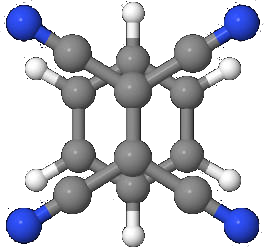
So let’s do this by example. Let us do the calculation for the density of states for a system we have used previously, Tetracyanoethylene Benzene, or TCNE-Benzene. This is compound molecule made up of two components: the TCNE and Benzene, here the TCNE is in front and the benzene is in the backgound (Fig. 1).

The CLUSTER file to run the calculation of this structure is:

GGA-PBE*GGA-PBE
GRP
          22  Number of inequivalent atoms
       0.0000      4.7079     -3.9776   1 ALL UPO
       0.0000     -4.7079     -3.9776   1 ALL UPO 
       4.0794      2.3559     -3.9732   1 ALL UPO 
      -4.0794      2.3559     -3.9732   1 ALL UPO
       4.0794     -2.3559     -3.9732   1 ALL UPO
      -4.0794     -2.3559     -3.9732   1 ALL UPO
      -4.1665      3.8824      2.9754   7 ALL UPO
       4.1665      3.8824      2.9754   7 ALL UPO
      -4.1665     -3.8824      2.9754   7 ALL UPO
       4.1665     -3.8824      2.9754   7 ALL UPO
       0.0000      2.6433     -3.9697   6 ALL UPO
       0.0000     -2.6433     -3.9697   6 ALL UPO
       2.2925      1.3220     -3.9702   6 ALL UPO
      -2.2925      1.3220     -3.9702   6 ALL UPO
       2.2925     -1.3220     -3.9702   6 ALL UPO
      -2.2925     -1.3220     -3.9702   6 ALL UPO
       0.0000      1.2969      2.9150   6 ALL UPO
       0.0000     -1.2969      2.9150   6 ALL UPO
      -2.3072      2.7100      2.9357   6 ALL UPO
       2.3072      2.7100      2.9357   6 ALL UPO
      -2.3072     -2.7100      2.9357   6 ALL UPO
       2.3072     -2.7100      2.9357   6 ALL UPO
       0.0000      0.0000 Net Charge and Moment

However, density of states is not a calculation that is normally done when you run NRLMOL, it has to be requested as a post-convergence calculation. That is, once the SCF cycle has converged, this calculation is now executed.

In order to request it, you have to set the option DOSOCCUV to ‘Y’ in the NRLMOL_INPUT.DAT file. For older versions of NRLMOL, you have to create an empty file called DOSOCCU to request the calculation.

So, to get the density of states calculated, you need the following:

The binary file (the program itself)
The CLUSTER file
Either the NRLMOL_INPUT.DAT with the option set or an empty file called DOSOCCU

Results¶

Once the program finishes, it should have generated a list of files called DOSO001, DOSO002, and so forth (one for every atom in the structure you ran, there should be 22 files for our case of TCNE-Benzene).

The files may also have other starting names (AF1O, AF2O, MINO, MAJO) depending on the type of calculation you set up.

So basically, we have a density of states file for every atom in our system that we must plot, but how do we know which file corresponds to what atom? Do we follow the order from the CLUSTER file? The answer is no, because NRLMOL orders the atoms once it processes the CLUSTER file.

However, remember that NRLMOL prints a file called XMOL.DAT which is basically an xyz file to visualize the molecule with Jmol[3] or any other molecular viewer, it contains a listing for the atoms calculated. The order of the atoms in this file is the same order followed by the DOS files.

Here is the contents of XMOL.DAT for our TCNE-Benzene:

   22
TCNE-Benzene
  0.00000    1.39877   -2.10067
  0.00000   -1.39877   -2.10067
  1.21314    0.69957   -2.10094
 -1.21314    0.69957   -2.10094
  1.21314   -0.69957   -2.10094
 -1.21314   -0.69957   -2.10094
  0.00000    0.68629    1.54255
  0.00000   -0.68629    1.54255
 -1.22092    1.43407    1.55350
  1.22092    1.43407    1.55350
 -1.22092   -1.43407    1.55350
  1.22092   -1.43407    1.55350
  0.00000    2.49131   -2.10485
  0.00000   -2.49131   -2.10485
  2.15872    1.24669   -2.10253
 -2.15872    1.24669   -2.10253
  2.15872   -1.24669   -2.10253
 -2.15872   -1.24669   -2.10253
 -2.20482    2.05448    1.57451
  2.20482    2.05448    1.57451
 -2.20482   -2.05448    1.57451
  2.20482   -2.05448    1.57451

As you can see from this listing, the atoms do not have the same order as in the CLUSTER file. Usually, NRLMOL orders atoms by listing carbons first, then hydrogens and the the rest of the atoms (it’s the standard ordering for molecules in Chemistry).

From the listing, we now know that the first 12 DOS files correspond to the carbons, files 13-18 correspond to the hydrogens and files 19-22 correspond to the nitrogens. So now we have to plot the DOS files for each of the components and for the full complex, but in order to do so we are going to need membership files.

Membership files¶

So far, we know that the DOSO files generated are for each atom in the system, and they follow the ordering from the XMOL.DAT file, so let’s put them side by side for clarity:

   22
TCNE-Benzene
  0.00000    1.39877   -2.10067 -> DOSO001
  0.00000   -1.39877   -2.10067 -> DOSO002
  1.21314    0.69957   -2.10094 -> DOSO003
 -1.21314    0.69957   -2.10094 -> DOSO004
  1.21314   -0.69957   -2.10094 -> DOSO005
 -1.21314   -0.69957   -2.10094 -> DOSO006
  0.00000    0.68629    1.54255 -> DOSO007
  0.00000   -0.68629    1.54255 -> DOSO008
 -1.22092    1.43407    1.55350 -> DOSO009
  1.22092    1.43407    1.55350 -> DOSO010
 -1.22092   -1.43407    1.55350 -> DOSO011
  1.22092   -1.43407    1.55350 -> DOSO012
  0.00000    2.49131   -2.10485 -> DOSO013
  0.00000   -2.49131   -2.10485 -> DOSO014
  2.15872    1.24669   -2.10253 -> DOSO015
 -2.15872    1.24669   -2.10253 -> DOSO016
  2.15872   -1.24669   -2.10253 -> DOSO017
 -2.15872   -1.24669   -2.10253 -> DOSO018
 -2.20482    2.05448    1.57451 -> DOSO019
  2.20482    2.05448    1.57451 -> DOSO020
 -2.20482   -2.05448    1.57451 -> DOSO021
  2.20482   -2.05448    1.57451 -> DOSO022

We can see from here that file DOSO0007 corresponds to the seventh carbon atom, file DOSO013 corresponds to the first hydrogen atom and so forth. As we previously stated, we need to generate three DOS plots: One for the full complex, one for the Benzene and one for the TCNE.

We clearly can see that the hydrogens belong to the Benzene and the nitrogens to the TCNE, but which carbons belong to the Benzene and which belong to the TCNE? we have no way of knowing this, so we need to open the XMOL.DAT file with Jmol to visualize the strucutre. Once you open it with Jmol, by positioning the cursor over a single atom it will tell you what number it is from the list, jot this number down and make a list for each atom of TCNE and benzene separately.

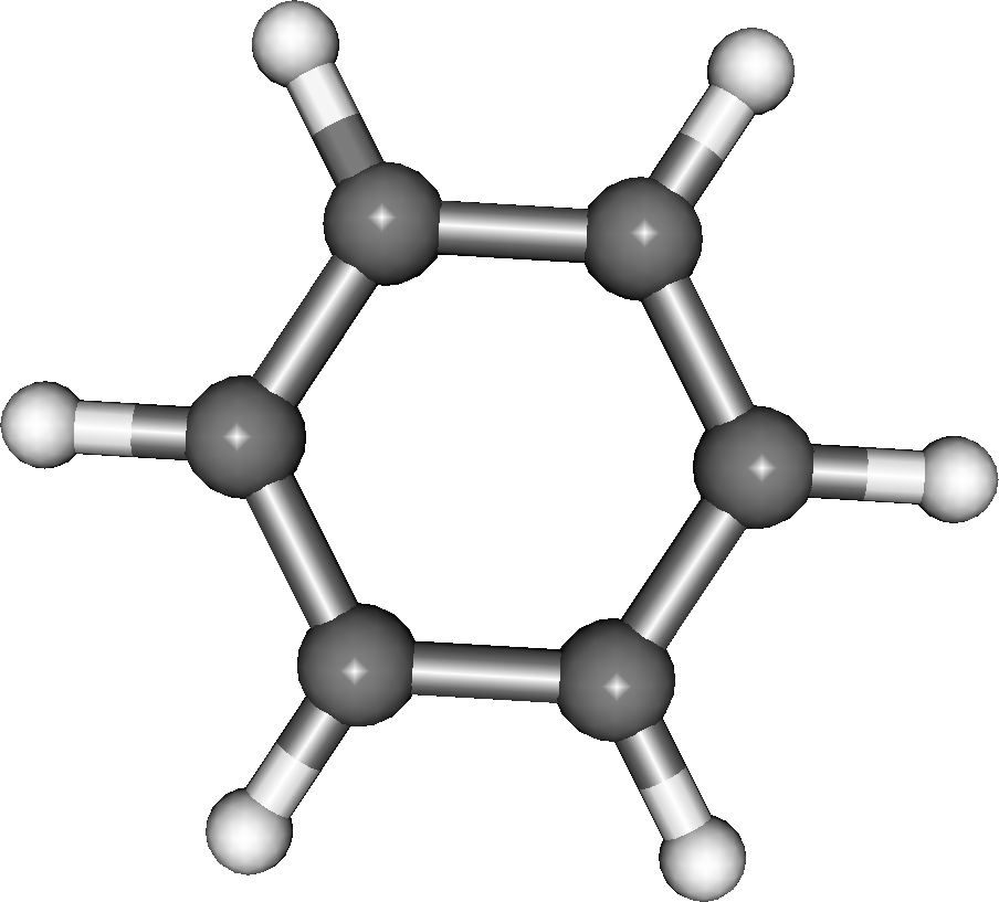
From this information you can create a membership list of the atom indexes for each of the substructures. For benzene, with the help of Jmol we know that carbon atoms 1-6 belong to the benzene and carbon atoms 7-12 belong to the TCNE. Therefore, the complete membership for benzene (fig. 2) is:

which are the indexes for the six carbon and the six hydrogen atoms.

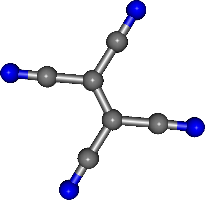
For TCNE (fig. 3) the membership is:

wich are the six carbon atoms and the four nitrogen atoms.

We must now use this listings to create the membership files for plotting the DOS for each substructure, we only need to put in the first line of the membership file the total atoms for that membership. The membership file for benzene (let’s call it benzene.mem) is:

In general, the ordering of the atom indexes is not necessary, it’s just shown here for clarity.

Similarly the membership file for TCNE (let’s call it tcne.mem) is:

Additionally, we must create the membership file for the full complex, this is trivial, as it is just a listing of the indexes of all the atoms in the structure (let’s call it total.mem), you can even generate it automatically with the computational tool of your choice.

Again the ordering is not important as long as each atom is listed.

We can now use these three membership files to plot their corresponding density of states.

Plotting¶

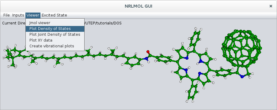
To plot the membership files, we use the NRLMOL_GUI program to do so. Set the project directory by selecting Set Project Directory from the File menu. This is the directory where you ran the calculation and that contains the DOS and other output files. After this, select Plot Density of States from Viewer in the main menu (fig. 4).

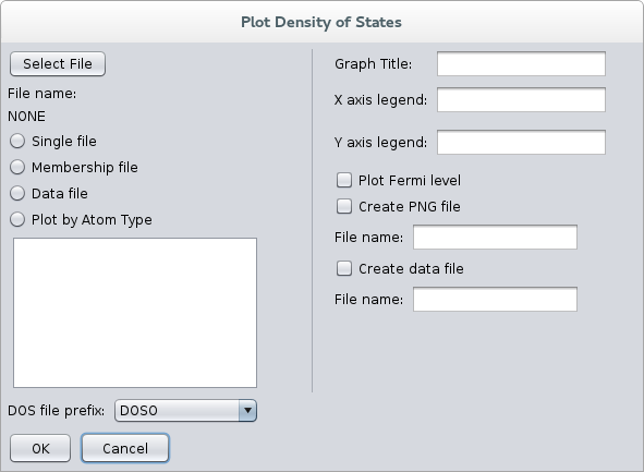
This will open the dialog box for plotting density of states (fig. 5), from here:

Press the “Select File” button to select the membership file you want to plot.
Select the “Membership file” radio button to process the file as a membership file.
Select the “DOS file prefix” to select the prefix of your DOS files (in case they are not named (DOSO)
Type the titles and axis legends for the graph.
Click on the checkbox if you want the Fermi level to be plotted (the file EVALUES must be present in the project directory).
You can select to write a graphics file output, although you can do that by doing a right-click on the plot window, this second option is preferred since you can do some adjustments to the graph before saving.
The last check mark Create data file should be checked, and a file name given (only when plotting from a membership file), no extension is required as it will automatically add .dat to the file name.

Why should a data file be created when plotting from a membership file? Well, the process goes as this: The program will take each of the DOS files for each atom, adds them together and puts it in a file for plotting, however; if you want to plot the data yourself with another program, you can use this data file for that purpose. After you are finished, you should now have three final data files:

benzene.dat a data file containing the DOS information for the benzene atoms generated from the benzene.mem file.
tcne.dat a data file containing the DOS information for the tcne atoms generated from the tcne.mem file.
total.dat a data file containing the DOS information for all the atoms generated from the total.mem file.

Let’s now use gnuplot[4] to generate the three plots in a single image from the data files.

Gnuplot usage¶

To now join together the three data files, we need to setup a gnuplot script to process the data in each file and plot them. However, we also need one extra data file for the Fermi level.

We get the Fermi level from the EVALUES file: open the file and look for the line containing FERMI LEVEL and the number next to it, the number is however given in Hartrees, so you must convert it to electron-volt by multiplying it by 27.2116. You could have also got it from the GUI, if you requested to plot the Fermi level, this goes and reads it from the file and puts in a pop up window so you can jot it down.

For the TCNE-Benzene this value is: -0.206529774179560 so its corresponding value in eV is -5.620005603

So make a file called fermi.dat and put this two lines in it:

-5.620005603 0
-5.620005603 70

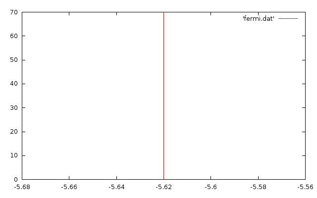
These are just two x,y pairs to be plotted. If you think about it, if the points are connected on a graph, they will generate a vertical line at the Fermi level (fig. 6). We give the second point a big y value (70 in this case, it can be naything) to make shure we cover all the plot surface.

Now we are ready to configure the plotting script for gnuplot. This is just a text file (let’s call it plot_sample.p) that conatins the following lines:

# This file will create a stacked plot for DOS
set terminal png size 1200,900 linewidth 3
set output 'DOSplot_sample.png'
set linestyle 1 linecolor rgb 'blue'
set linestyle 2 linecolor rgb 'red'
set multiplot layout 3,1
# first plot top
set bmargin at screen 0.65
set tmargin at screen 0.95
set xrange[-12:0]
set yrange[0:10]
set xtics format ' '
set ytics 0,2,8
plot 'tcne.dat' with lines linestyle 1 notitle,'fermi.dat' with lines linestyle 2 notitle
# Second plot middle
set bmargin at screen 0.35
set tmargin at screen 0.65
plot 'benzene.dat' with lines linestyle 1 notitle,'fermi.dat' with lines linestyle 2 notitle
# Third plot
set bmargin at screen 0.05
set tmargin at screen 0.35
set xtics format '%g'
plot 'all.dat' with lines linestyle 1 notitle,'fermi.dat' with lines linestyle 2 notitle
unset multiplot

Lines that begin with # are comments and are thus ignored. The configurable options are:

We set a terminal output of png, this means we will generate a .png graphic file
The requested linewidth is 3 is needed for publication qualitiy graphs.
The set output line specifies the file name of the generated file.
Two linestyles are defined, which specify the line colors for the DOS data and Fermi level respectively.
We remove unnecessary data by adjusting the x range (usually on the unoccupied states) to the left of the Fermi level (set xrange[-12:0]).
We adjust the y range so all plots have the same height (set yrange[0:10]).
We remove any number on the x axis until the last plot with: set xtics format ‘ ‘
The set ytics 0,2,8 means that the y range will be printed from 0 to 8 in increments of 2.
You can change the order of the plots by specifying the name of the .dat file in each section (just don’t forget to include the fermi.dat file).

Once you set this up, run the script through gnuplot with the folowing command (in Linux, other platforms are untested):

gnuplot plot_sample.p

You may need to run this command several times, while adjusting the values in the gnuplot script.

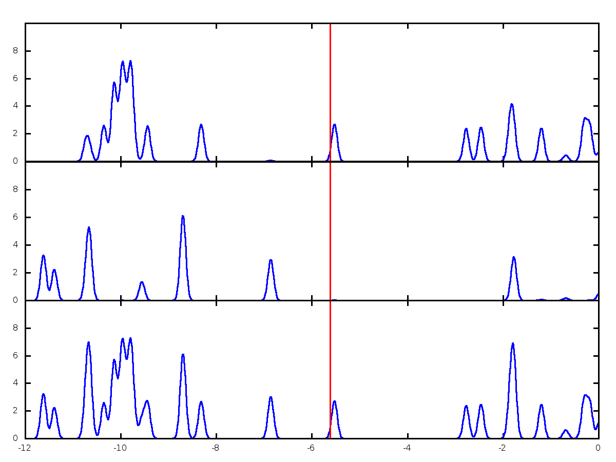
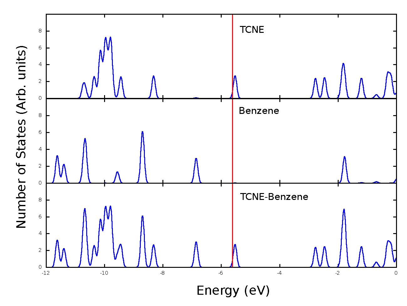
Once you get plot you’re confortable with (fig. 7), you still need to include the Axis labels as well as the descriptions of the individual plots (what part of the molecule each section represents), this can be done with any graphical editor (in the lab I usually use the GIMP[5] package, but it can be done with a presentation editor) to edit the png file (fig. 8).

Bibliography¶

David S. Sholll & Janice A. Steckel, Density Functional Theory: A practical Introduction, Wiley (2009).
Ricahrd M. Martin, Electronic Structure, Basic Theory and Practical Methods, Cambridge University Press (2013).
Jmol: An open-source Java viewer for chemical structures in 3D. http://www.jmol.org
gnuplot: A portable command-line driven graphing utility. http://www.gnuplot.info
GIMP: The GNU Image Manipulation Program. http://www.gimp.org

Plotting density of states using NRLMOL¶

Introduction¶

Setup¶

Results¶

Membership files¶

Plotting¶

Gnuplot usage¶

Bibliography¶

Table Of Contents

Previous topic

Next topic

This Page